(2008/06/24)
Atlantis Blueprintに触発された。聖地ネットワークのポイントに10Φが使われている。緯度16.18。
10Φがあるならば、0.1Φ=0.1618。これは、fitvalの漸近値に近い?
(2007/xx/xx) fitvalの漸近値が数学定数の組み合わせでできないかを検討したことがあるが、不発。
今度は何を調べるか、、、
π(3.1415...)、e(2.718...)、Φ(1.618...)に関して、少数部の数分布を調べて見ることにする。
分布といってもいろいろあります。2008/06/25)
[1]100,1000,10000,...とかの区間の合計をグラフ化した場合
[2]区間平均?
[3]@@@中断@@@:メモ参照で整理要!
fitvalの誤差部分の傾向に類似すれば、おもしろい。
(2008/06/24)It was touched off by Atlantis Blueprint. 10Φ is used for the point on the sacred ground network. Latitude 16.18. 0.1Φ=0.1618 if there is 10Φ. Is this near an asymptotic value of fitval?(2007/xx/xx) The misfire though whether an asymptotic value of fitval cannot be done by combining mathematics constants has been examined.
What do you examine this time?Small number of people will examine the cloth for a few minutes of the part for π(3.1415...), e(2.718...), and Φ(1.618...) and it see. It is variously even if it is said that it distributes. 2008/06/25)[1]Section..total..graph.[2]Section average?[3]@@@ interruption @@@: It is a memo reference and an arrangement main point.
If it resembles the tendency in the error margin part of fitval, it is interesting.
end
2008年6月30日月曜日
狩猟型読書
(2008/06/16)
サイトで記事発見!
キーワードとして、記録。
直感を鍛えるにはいいかも。サイトが消える前に抜粋!
http://www.nikkeibp.co.jp/style/biz/saitotakashi/080613_23rd/
~~~
ポイントは、どんなキーワードに目をつけるか、にある。冒頭からじっくり読み込んでいくのではなく、アンテナを張って必要な言葉だけをキャッチしていく。自分で森の中をさまよって獲物を探し回るというより、「ここだ」と思う場所に網を張って虎視眈々と待つ、という感じに近い。実際に読むのは視覚だが、そこで問われるのは動物的な嗅覚、まさに直感である。ではその感度をいかに高めるかといえば、これは何度も繰り返して慣れていくしかない。毎日のように、何冊でもチャレンジしてみていただきたい。この方法に慣れてくると、むしろキーワードのほうから自然に目に飛び込んでくるようになる。獲物が勝手に網に引っかかってくれるわけだ。おかげで、読むスピードは格段にアップする。あるいは、関連するキーワードまで目に入るようになる。知識の幅が広がるわけだ。
2008年6月29日日曜日
過去の叡智を求めて(1)
For past wisdom(1)
KI図書館)普段行かないコーナーで発見!
[1]:ほぼ、読み完了
アトランティス・ブループリント―神々の壮大なる設計図 (知の冒険シリーズ) (単行本) コリン ウィルソン (著), ランド フレマス (著), Colin Wilson (原著), Rand Flem‐Ath (原著), 松田 和也 (翻訳)
The Atlantis Blueprint/Rand Flem-Ath, Colin Wilson
[2]:読み未完、現在進行形?
アトランティスの暗号―10万年前の失われた叡智を求めて (単行本) コリン ウィルソン (著), Colin Wilson (原著), 松田 和也 (翻訳)
Atlantis and the Kingdom of the Neanderthals/100,000 Years of Lost History by Colin Wilson
~~~
私的には、[1]がすっきり明快なにに対して、[2]は断片的な話を盛り込みすぎて、読者をオカルティックな世界に置き去りにして終わりそうな雰囲気である。
Privately, [1] lucidly refreshingly confronts,[2]A fragmentary story is included too much, it leaves in the field of the reader of ..Ocalticc.. Yo, and the atmosphere that seems to end.
~~~
(2008/06/21)
ブループリントの骨子)
ノア洪水以前の知識
10万年前の高度文明
フリーメーソンをこれを探している?
地球をΦの単位で分割し、ランドマークをたてた。ピラミッドもその一つ。
その後、急激な地殻変動で崩壊。
痕跡が、南極の氷の下とか未開の地にのこる、、、
Substance of blue print)
Knowledge before flood of Noah
Advanced civilization 100,000 years ago
Is it looked for the Freemason and is it looked for this?
The earth was divided by the unit of Φ, and the landmark was set up. The pyramid is the one.
Afterwards, it collapses because of rapid diastrophism.
Signs remain in the under of the ice of the South Pole or the undeveloped region.
~~~
聖地ネットワークをGoogleMapでチェックするプロジェクトがあれば、、、
If there is a project to check the sacred ground network with GoogleMap,...
~~~
Blueprint:青写真、設計図とか。
end
渋滞学:流量-密度グラフの意味(7)
キーワードは、
[1]速度と視野角
[2]前車との相対関係
視野角での有効視野面積に占める 前車の形状の占有面積を
経験から、速度に関係なく、相対値で保持する傾向があることが判明した。
ベテランと初心者のドライバで、ばらつきがあるが、
前車との追従運転により、時間の経過とともに、適正値に落ち着くものと
考えられる。
The key word is
[1]Speed and viewing angle
[2]Relative relation to preceding vehicle
It turned out to tend to maintain the occupation area of shape in the preceding vehicle that occupied it to the effective view area in the viewing angle from the experience by a relative value regardless of the speed.
Though it is uneven in the old-timer and beginner's driverIt is thought that it settles down in a proper value with the time passage by the follow driving with the preceding vehicle.
~~~
この考えで、車間警告機能を実現できる、、、
The warning function between cars can be achieved by this idea.
~~~
(google検索:時速 視野角)
(google検索:車速 視野角)
で、検索したら、短時間であるが以下が引っかかった。
TODO)内容のチェック要!
(google retrieval: Per hour viewing angle)
(google retrieval: Viewing angle of velocity of car)
The following were caught though a short time when .... retrieving it.
TODO) Check main point of content.
~~~
[1]
http://www.denso.co.jp/ja/aboutdenso/technology/dtr/v12_1/files/18.pdf
運転者の視覚認知機能の解明とモデル化の研究
Clarification of driving person's sight acknowledgment function and research of modeling
2008/06/30追記)
ドライバは先行車の視覚的な面積変化をもって接近・離間検出をおこなっているという仮説のもと、「ドライバは前車との車間距離変化を前車の視覚的面積変化として認識し加減速操作をおこなっている」
とあるが、視野角との関係には、明確に言及していない。
The driver is original of the hypothesis of having a visual area change of the proceeding vehicle and doing the approach and the alienation detection. The driver recognizes the distance change between cars with the preceding vehicle as a visual area change in the preceding vehicle and is operating the addition and subtraction velocity.
The relation to the viewing angle is not clearly referred.
~~~
[2]
http://www.j-tokkyo.com/2002/H04N/JP2002-152718.shtml
【発明の名称】 画像処理装置
【 title of invention 】Image processor
【発明者】 【氏名】山田 正博
【要約】 【課題】画像処理のためにメモリに格納する画像データの量を少なくし、かつ必要な画像を得る。
【発明の詳細な説明】【0001】
【発明の属する技術分野】本発明は、車両のルームミラーの位置等に取り付けたビデオカメラにより撮像した前方の道路状況を画像処理し、レーンマークや車両等を検出する画像処理装置に関する。
This invention processes the road situation of which it takes picture with the video camera installed in the position etc. of the room mirror of the vehicle forward in the image, and concerns the image processor that detects the lane mark and the vehicle, etc.
@@@
本発明では走行速度に応じて視野角を変更する。
@@@
また、図4に示すように、走行速度に応じて線形に連続的に視野角を変化させることもできる。図4は車速に対する視野角の変化の一例を示したグラフである。横軸は車速を表す時速であり、縦軸は視野角を表す。この例では時速40km/hのときに視野角を30°とし、それより速くなると視野角は小さくなり、遅くなると視野角は大きくなる。
Moreover, the viewing angle can be changed linear continuously by responding at the running speed as shown in Figure 4. Figure 4 is a graph where one example of the change in the viewing angle into the velocity of the car was shown. A horizontal axis is per hour which the velocity of the car is shown, and the spindle shows the viewing angle. When it becomes small, and the viewing angle slows when the viewing angle is assumed to be 30° in this example at the time of 40 km/h in per hour, and it quickens more than it, the viewing angle grows.
【出願人】【識別番号】000237592【氏名又は名称】富士通テン株式会社
【 those who apply 】【 name or name 】 Fujitsu Ten of 【 identification number 】000237592 Ltd.
~~~
[3]
http://www.j-tokkyo.com/2006/B60R/JP2006-182324.shtml
【発明の名称】 車両用警報装置
【 title of invention 】Alarm device for vehicle
【発明者】 【氏名】服部 彰
【住所又は居所】愛知県豊田市トヨタ町1番地 トヨタ自動車株式会社内
【 address or address 】In TOYOTA MOTOR CORPORATION one in Aichi Prefecture Toyota City Toyota town
【要約】 【課題】運転者の警報対象物についての認識遅れを緩和する車両用警報装置を提供すること。
Offer the alarm device for the vehicle where the recognition delay of driving person's warning object is eased.
TODO)特許の中身は見れないのか?見れたような、、、図が見たい!
~~~
TODO)レイノルズ数算出試行時の計算値を挿入する。メモ整理要!、当面、保留!
~~~
end
2008年6月28日土曜日
渋滞学:流量-密度グラフの意味(6)
Congestion study: Meaning of flowing quantity-density graph(6)
2008/06/21~2008/06/25)
とうとう、ゴールが見えてきました。
~~~
速度と視野角の関係は、
(速度と視野の広さ)視力0.1以上の範囲
The relation between the speed and the viewing angle
(speed and area of view)Eyesight is a range of 0.1 or more.
40 km/h -100 dgrees
70 km/h -65 dgrees
100 km/h-40 dgrees
とある。
~~~
100 km/h の時の車間:40m がメタ安定に近づいた値とすると、
前車の位置における有効視野面積に対する前車の占有面積の比率を求める。
※ここでは、 面積を円形として捉えている。楕円という考えもできるかも。
When assuming the value for 100km/h, 40m between cars to approach a steady meta, The ratio of the occupation areas of the preceding vehicle in the position of the preceding vehicle to the effective view area is requested.
- Here, the area is caught as a circle. Can you think, that is, the oval?
有効視野面積(A)=(車間*TAN(RADIANS(視野角度/2)))^2*PI()
前車の占有面積(B)=(車間*TAN(前車の幅の半分/車間))^2*PI()
比率(R)=前車の占有面積(B)/有効視野面積(A)
なお、前車の幅を 2m とした。
{Effective view area}(A)=({Between cars}*TAN(RADIANS({Viewing angle degree}/2)))^2*PI()
{Occupation area of preceding vehicle}(B)=({Between cars}*TAN({Half of width in preceding vehicle}/{Between cars}))^2*PI()
R=B/A
or
A=(TAN(RADIANS({Viewing angle degree}/2)))^2
B=(TAN({Half of width in preceding vehicle}/{Between cars}))^2
R=B/A
Width in the preceding vehicle was assumed to be 2m.
***
A(m^2)=(40*TAN(RADIANS(40/2)))^2*PI()=665.89
B(m^2)=(40*TAN(1/40))^2*PI()=3.14
R=3.14/665.89=47.2e-4
or
R=(TAN(1/40))^2/(TAN(RADIANS(40/2)))^2
***
他の速度で、R=47.2e-4 に近くなるように、車間を手で微調整した結果、以下となった。
It fine-tuned between cars by the hand to become near R=47.2e-4 other speeds, therefore it became it as follows.
他の速度の場合の視野角の情報がないが、上記の3点の線形?として
以下とした場合で、比率:Rを求める。
Is it the above-mentioned linear though there is no information on the viewing angle for other speeds in three points?The ratio when it is time when it made it as follows ..making it..: R is obtained.
 X軸:速度(km/h) ,speed
Y軸:視野角(dgrees) ,Viewing angle
~~~
これから、基本図を作成するために、密度と流量を求める。
密度(台/km)=1000(m)/車間(m)
流量(台/5mins)=密度(台/km)*速度(km/h)/(60/5)
Hereafter, to make a basic chart, the density and flowing quantity are requested.
density(cars/km)=1000(m)/{Between cars}(m)
{flowing quantity}(cars/5mins)=density(cars/km)*speed(km/h)/(60/5)
とうとう、ゴールが見えてきました。
~~~
速度と視野角の関係は、
(速度と視野の広さ)視力0.1以上の範囲
The relation between the speed and the viewing angle
(speed and area of view)Eyesight is a range of 0.1 or more.
40 km/h -100 dgrees
70 km/h -65 dgrees
100 km/h-40 dgrees
とある。
~~~
100 km/h の時の車間:40m がメタ安定に近づいた値とすると、
前車の位置における有効視野面積に対する前車の占有面積の比率を求める。
※ここでは、 面積を円形として捉えている。楕円という考えもできるかも。
When assuming the value for 100km/h, 40m between cars to approach a steady meta, The ratio of the occupation areas of the preceding vehicle in the position of the preceding vehicle to the effective view area is requested.
- Here, the area is caught as a circle. Can you think, that is, the oval?
有効視野面積(A)=(車間*TAN(RADIANS(視野角度/2)))^2*PI()
前車の占有面積(B)=(車間*TAN(前車の幅の半分/車間))^2*PI()
比率(R)=前車の占有面積(B)/有効視野面積(A)
なお、前車の幅を 2m とした。
{Effective view area}(A)=({Between cars}*TAN(RADIANS({Viewing angle degree}/2)))^2*PI()
{Occupation area of preceding vehicle}(B)=({Between cars}*TAN({Half of width in preceding vehicle}/{Between cars}))^2*PI()
R=B/A
or
A=(TAN(RADIANS({Viewing angle degree}/2)))^2
B=(TAN({Half of width in preceding vehicle}/{Between cars}))^2
R=B/A
Width in the preceding vehicle was assumed to be 2m.
***
A(m^2)=(40*TAN(RADIANS(40/2)))^2*PI()=665.89
B(m^2)=(40*TAN(1/40))^2*PI()=3.14
R=3.14/665.89=47.2e-4
or
R=(TAN(1/40))^2/(TAN(RADIANS(40/2)))^2
***
他の速度で、R=47.2e-4 に近くなるように、車間を手で微調整した結果、以下となった。
It fine-tuned between cars by the hand to become near R=47.2e-4 other speeds, therefore it became it as follows.
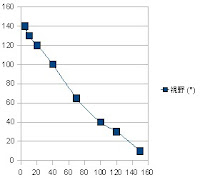
速度(km/h) speed | 視野角(degrees) Viewing angle | 車間(m) between car | 速度(m/s) speed | R(1e-4) |
40 | 100 | 12.25 | 11.11 | 47.13 |
70 | 65 | 22.85 | 19.44 | 47.25 |
100 | 40 | 40 | 27.78 | 47.2 |
他の速度の場合の視野角の情報がないが、上記の3点の線形?として
以下とした場合で、比率:Rを求める。
Is it the above-mentioned linear though there is no information on the viewing angle for other speeds in three points?The ratio when it is time when it made it as follows ..making it..: R is obtained.
 X軸:速度(km/h) ,speed
Y軸:視野角(dgrees) ,Viewing angle
~~~
速度(km/h) speed | 視野角(degrees) Viewing angle | 車間(m) between car | 速度(m/s) speed | R(1e-4) |
5 | 140 | 5.37 | 1.39 | 47.11 |
10 | 130 | 6.85 | 2.78 | 47.01 |
20 | 120 | 8.45 | 5.56 | 47.12 |
40 | 100 | 12.25 | 11.11 | 47.13 |
70 | 65 | 22.85 | 19.44 | 47.25 |
100 | 40 | 40 | 27.78 | 47.2 |
120 | 30 | 54.35 | 33.33 | 47.16 |
150 | 10 | 166.5 | 41.67 | 47.13 |
これから、基本図を作成するために、密度と流量を求める。
密度(台/km)=1000(m)/車間(m)
流量(台/5mins)=密度(台/km)*速度(km/h)/(60/5)
Hereafter, to make a basic chart, the density and flowing quantity are requested.
density(cars/km)=1000(m)/{Between cars}(m)
{flowing quantity}(cars/5mins)=density(cars/km)*speed(km/h)/(60/5)
速度(km/h) speed | 車間(m) Between cars | 密度(台/km) density(cars/km) | 流量(台/5mins) flowing quantity(cars/5mins) |
5 | 5.37 | 186.39 | 77.66 |
10 | 6.85 | 145.99 | 121.65 |
20 | 8.45 | 118.34 | 197.24 |
40 | 12.25 | 81.63 | 272.11 |
70 | 22.85 | 43.76 | 255.29 |
100 | 40 | 25 | 208.33 |
120 | 54.35 | 18.4 | 183.99 |
150 | 166.5 | 6.01 | 75.08 |
 X軸:密度(台/km) ,density(cars/km)
Y軸:流量(台/5mins) , flowing quantity(cars/5mins)
あとは、これに運転手の習熟度合いで、バラツキが発生するグラフになる。
It becomes a graph where the difference is generated by being in this the proficiency combination of the driver.
end
渋滞学:流量-密度グラフの意味(5)
2008/06/21)
再度、方向転換?
渋滞学、p.46)基本図の傾向を探るは変更なし。
制動距離の考えから離れる。
Again, turnabout?The congestion study and p.46) It is ..search.. change none as for tendency in a basic chart. It parts from the idea of the slip distance for brake.
~~~
人は車間をどのように判断しているのか?
高速道路から一般道路に入ったときの、速度間隔が鈍るのは、、、
How is the person judging between cars?The speed interval's when entering the public highway from the expressway becoming duller
~~~
相対速度、、、
速度に応じて、視野が狭まる
視野の中における前車の占有面積の割合から、車間を判断しているのでは?
Relative speed...View narrows responding at the speed. Is it judged from the ratio of the occupation area of the preceding vehicle in view between cars?
~~~
よもや、制動距離を意識して、車間をとっているのではない、、、
It doesn't take between cars considering the slip distance for brake possibly.
~~~
ここから、速度と視野の関係を調べはじめる。
It begins to examine the relation between the speed and view from here.
2008/06/21)
車きました。仕事終電です。日曜日も出です。何か、eventがここでは圧縮されてきました。WOOOO...
end
渋滞学:流量-密度グラフの意味(4)
2008/06/17)
方針転換?
***
Reを導き出す?のは中断!した感がある。復活できるか?かなり、落ち込んでいます。
渋滞学、p.46)の基本図の傾向は、どのようなルールなのか?
***
渋滞学、p.48)
「車間距離40km/hで渋滞が発生する。
1車線、密度=25台/kmで、車間=40m
自由走行している車が急ブレーキを踏んでギリギリ止まれる制動距離に等しい。」
と記述あり。
Congestion study and p.48)「Congestion occurs at the distance 40 km/h between cars. It is equal to the slip distance for brake that hits the brakes with 1 lane and density =25/the km by the car that freely runs =40m between cars and can stop in the very limit. 」 It describes and it exists.
~~~
速度と制動距離の関係から、基本図ができているのか?
Does a basic chart consist of the relation between the speed and the slip distance for brake?
~~~
密度低い~メタ安定までは、制限時速(100km/h?)で制限されているような。
メタ安定後、渋滞になるまでの車間のルールは?
Density low. Will not be limited the meta with stability by limitation per hour (100 km/h?). The rule between cars to becoming after meta stabilizes congestion?
~~~
車間に関して、
車が一秒間に進む距離(m/s)と
制動距離との関係は見えない。
For between carsThe car will not see the relation between advanced distance (m/s) and the slip distance for brake in one second.
~~~
逆に、制動距離を意識して走行していないような、車間が短い、、、
Oppositely, it is short between cars not running considering the slip distance for brake.
@@@
自分の場合で考えるとそうかも、、、低速?走行しているので、、、、(燃費走行とも言える?)
@@@
~~~
検索して、「車間の2秒ルール」を知りました、、、
It retrieved, and it knew "Rule for two seconds between cars".
end
渋滞学:流量-密度グラフの意味(3)
2008/06/xx)
車速は、以下の式と、渋滞学:p.46のグラフから求められる。
流量(台/h)=速度(km/h)×密度(台/km)
逆算した結果が何を意味しているのか?
この作業は、何を目的にしているのか? 不明確になりつつあった。
~~~
2008/06/26):補足
Re=(密度ρ×流速u×直径d)/粘性係数μ
流量(台/h)=速度(km/h)×密度(台/km)
から、
Re=(流量×直径d)/粘性係数μ
直径、粘性係数=一定ならば、Reは、流量に比例する。
~~~
車は、渋滞すると、空気みたいに圧縮して速度を増すことにはならないので、
速度は頭打ちになる。
つまり、
流量が何とか以上が乱流とかは定義できない、、、
end
渋滞学:流量-密度グラフの意味(2)
2006/06/12~)
ここから、レイノルズ数を求める試み)
円管の場合)
Re=(密度ρ×流速u×直径d)/粘性係数μ
Re:レイノルズ数、単位なし
ρ:kg/m^3
u:m/s
d:m
μ:Pa・s
あるいは、
Re=(流速u×直径d)/動粘性係数ν
ν:m^2/s
~~~
車の場合は、それぞれ何になるか?
車線は限定で、それ以外に行きようがないので、管内に近い、、、?
強引に、※これは頭の体操か?
密度ρ(kg/m^3) :密度(台/km)?
:車の重さ関係する? 平均:>1t?、大型車、小型車とか。
流速u(m/s) :車の速度(km/h)?
直径d(m) :車線の幅(m)?
~~~
Re=2300で、粘性係数を逆算してもしたりした。同様に、動粘性係数も逆算できる、、、か。
粘性係数を求めても何か意味があるか?
~~~
DO図書館)
道具としての流体力学 (単行本) 山口 浩樹 (著), 松本 洋一郎
p.22で、液体、気体の粘性係数の表あり。
計算した?自由走行の粘性係数を比較した。
結果は?:ひまし油に近い?とか、計算違い???:何かあやしい、、、
***
p.22)
粘性係数(1e-6 Pa・s)
空気 :18.2
***
p.66)
温度290K、動粘性係数(m^2/s)
水 :1.14e-6
空気 :14.6e-6
人・車 :更に大きい値???
***
密度(kg/m^3)
空気 :1.2
ヘリウム:0.18
水 :1000
~~~
end
お手軽画像編集
紙ベースの資料を部分的にプログに貼り付けようとした場合)
ものとしては、全体のイメージが分かればよいという品質を前提。
[1]いままでは、スキャナーで取り込み、画像編集ソフトで加工し、アップロードする流れ。
はじめは面白くでやっていることでも、繰り返すうちに、苦痛?億劫になる。
[2]携帯電話で写真をとり、PCにUSBで接続し、それから。。。
作業するPCが変わる場合があり(会社・自宅、ノートPC、vmwareだったりと)、ちょっと
画像調整 したいのに、それぞれに重装備の画像編集ソフト(Photosopとか)をインスト
するのは、避けたい。
※いま使っている、vmwareのHDDの空きが少なく、整理する時間もないので、
vmwareに追加ディスクを設定すればという話もあるが、極力、現状維持で、
目的の作業だけに集中したいとする。
~~~
要件としては、写真の加工で、芸術作品のようなイメージ作成ではないので。
・トリミング
・回転
・若干の補正:明暗、コントラスト
ができればいいとする。デジカメ画像編集としての一般的な要件です。
とりあえず、画像編集で軽めのフリーソフトを探していたら、
「2007/04/11、Photoshopのウェブアプリ版が無料公開予定」を発見!
早速ベータに登録、特に違和感なく、画像編集できました。すばらしい!!!
これで、会社でも家でも、携帯から画像を転送し、好きなPCで作業できます。感謝!
http://www.photoshop.com/express/
~~~
プロフィール画像の加工がずっと仕掛かっていたので、とり頭イメージから鉛筆で書いて
もらったのを携帯でとって、「Photoshop Express」で加工したものが以下。
 このままでもいいが、画像編集・変換ソフトの探索で見つけた「絵師のえそらごと」を試す。
写真を油絵風にするもの。
http://www.esola.co.jp/index.html
バージョン:4.02、無償版で試す。有償版もありました。
絵師:くりで変換したものが以下。処理はエンドレス?で続くので、途中で止めましたが。
なにやら、すばらしい作品ができた模様です。
そんなわけで、この変換画像を登録しました。
 どうですか?
渋滞学:流量-密度グラフの意味(1)
Congestion study: Meaning of flowing quantity-density graph(1)
またまた、わき道にそれました。
貧乏ひまなし状態と15年ぶりに車購入で、資金難のために、6月のエネルギーを
使い果たしました。
が、素数の探求で何かやろうとはしています。
今回は、渋滞学です。
思考期間:2008/06/12~2008/06/25、この後、メモ整理。頭の冷却期間、、、続く。
DO図書館):再読
渋滞学 (新潮選書) (単行本) 西成 活裕 (著)
p.46)基本図?:人型、ラムダ型とも言われている。
貧乏ひまなし状態と15年ぶりに車購入で、資金難のために、6月のエネルギーを
使い果たしました。
が、素数の探求で何かやろうとはしています。
今回は、渋滞学です。
思考期間:2008/06/12~2008/06/25、この後、メモ整理。頭の冷却期間、、、続く。
DO図書館):再読
渋滞学 (新潮選書) (単行本) 西成 活裕 (著)
p.46)基本図?:人型、ラムダ型とも言われている。

感じとしては、密度低い~メタ安定までは、層流で、メタ安定~密度高い方は、乱流に見える。
自由走行でのメタ安定部分は、レイノルズ数=2300近辺になるのか?それとも、、、
As feeling, density low. Meta stability to meta stability because of laminar air flow?Density high looks like the war. Does the meta stability part in a free running become about Reynolds number =2300?Or,
~~~
結論として、レイノルズ数の割出には失敗したが、
グラフの傾向線に近似したルールを発見できた。後述する。
In conclusion, the rule approximated to the trend line in the graph was able to be discovered though it failed in the crack going out of the Reynolds number. It describes it later.
end
2008年6月4日水曜日
遺伝子分布の傾向をみる(1-4) 、データ取得:NIH,Dog
ヒトゲノムではなく、「UCSC Genome Bioinfomatics」で得たDogの遺伝子配置が正規分布にならなかったので、NIHで探した。
~~~
(1)
http://research.nhgri.nih.gov/dog_genome/
ftp://ftp.ncbi.nih.gov/genomes/Canis_familiaris/
ftp://ftp.ncbi.nih.gov/genomes/Canis_familiaris/Assembled_chromosomes/
染色体1番=cfa_chr1.agp.gz
ありました。
===
展開すると、chr1.agp
抜粋すると、
#
# Canis familiaris chromosome 1, whole genome shotgun sequence
#
# This file provides assembly instructions for sequence NC_006583.2
# included in reference assembly of NCBI build 2 (Dog2.0 May 2005).
#
#chrom chr_start chr_stop part_no part_type comp_id/gap_len comp_type/gap_type comp_end/linkage orientation/empty
chr1 1 3000000 1 N 3000000 clone no
..............
から、「chr_start chr_stop 」の2項目の数字を、OpenOffice OpenDocument表計算でCSV形式にする。
~~~
(2)
染色体を変更して、同様にCSV形式のファイルを作成する。
~~~
(1)
http://research.nhgri.nih.gov/dog_genome/
ftp://ftp.ncbi.nih.gov/genomes/Canis_familiaris/
ftp://ftp.ncbi.nih.gov/genomes/Canis_familiaris/Assembled_chromosomes/
染色体1番=cfa_chr1.agp.gz
ありました。
===
展開すると、chr1.agp
抜粋すると、
#
# Canis familiaris chromosome 1, whole genome shotgun sequence
#
# This file provides assembly instructions for sequence NC_006583.2
# included in reference assembly of NCBI build 2 (Dog2.0 May 2005).
#
#chrom chr_start chr_stop part_no part_type comp_id/gap_len comp_type/gap_type comp_end/linkage orientation/empty
chr1 1 3000000 1 N 3000000 clone no
..............
から、「chr_start chr_stop 」の2項目の数字を、OpenOffice OpenDocument表計算でCSV形式にする。
~~~
(2)
染色体を変更して、同様にCSV形式のファイルを作成する。
遺伝子分布の傾向をみる(1-3) 、データ取得:WhoGA(Rice)
[3]日本:イネの遺伝子 Rice - Oryza sativa GBrowse - Map View Build 04 http://rgp.dna.affrc.go.jp/whoga/download.html
染色体上の遺伝子位置のデータを取得する方法を示す。
~~~
(1)
ページ下部の「All annotatied results」で、参照したい染色体を「File」の「gff file」
からダウンロードする。
~~~
(2)
例)染色体1番=PREDICTED_GENESET_CHR01_all.gff になる。
ファイルの先頭を抜粋すると、
:見出しはない。
===
chr1 mRNA gene 2449 8671 . + . gene_id "OSJNOa264G09.1";
......
4項目、5項目目が、遺伝子の開始、終了と思われる。
(3)
対象項目をOpenOffice OpenDocument表計算でCSV形式にする。
~~~
(4)
染色体を変更して、同様にCSV形式のファイルを作成する。
遺伝子分布の傾向をみる(1-2) 、データ取得:UCSC
[2] UCSC Genome Bioinfomatics
http://hgdownload.cse.ucsc.edu/downloads.html
染色体上の遺伝子位置のデータを取得する方法を示す。
~~~
(1)
VERTEBRATES - Complete annotation sets
で、参照したい対象生物を選択する。
~~~
(2)
例)ヒトの場合、「Human」を選択する。
~~~
(3)
「Full data set」を選択。
~~~
(4)
先頭のファイル:chromAgp.zip をダウンロードする。
※これ以外のファイルに関しては、内容未確認! ※TODO※
~~~
(5)
chromAgp.zipを展開すると、染色体ごとのファイルができる。
例)染色体1番=chr1.agp ※テキストエディタで開ける。
chr1.agp の先頭を抜粋する。
:見出しはなく、生データがそのまま。
===
chr1 1 616 1 F AP006221.1 36116 36731 -
chr1 617 167280 2 F AL627309.15 241 166904 +
......
2項目、3項目目が遺伝子の開始位置、終了位置であると思われる。
~~~
(6)
2項目、3項目目を、OpenOffice OpenDocument表計算でCSV形式にする。
~~~
(7)
対象生物を変更して、同様にCSV形式のファイルを作成する。
遺伝子分布の傾向をみる(1-1) 、データ取得:NIH
[1]米国:有名なNIH Human Genome Resources (ヒトゲノム) http://www.ncbi.nlm.nih.gov/genome/guide/human/
染色体上の遺伝子位置のデータを取得する方法を示す。
~~~
(1)
左図の染色体で、参照したいものを選択する。
Browse your Genome Click on the Chromosome to show
~~~
(2)
例)染色体1番の場合、以下のURLとなる。
http://www.ncbi.nlm.nih.gov/mapview/maps.cgi?ORG=hum&MAPS=ideogr,est,loc&LINKS=ON&VERBOSE=ON&CHR=1
~~~
(3)
ページ下部の「Map 3: Genes On Sequence 」で「Table View」 を選択することで、
http://www.ncbi.nlm.nih.gov/mapview/maps.cgi?TAXID=9606&CHR=1&MAPS=ideogr,ugHs,genes[1.00%3A247249719.00]&CMD=TXT#1
~~~
(4)
ページ右上の「Download Data」を選択することで、画面の情報をテキスト形式でダウンロードできる。
~~~
(5)
(3)で、ページ上部の「Chromosome: [ 1 ] 2 3 4 5 6 7 8 9 10 11 12 13 14 15 16 17 18 19 20 21 22 X Y MT 」で、別の染色体を見る場合は、対象の番号を選択する。
~~~
(6)
取得したテキスト(先頭を抜粋)を示す。
===
Homo sapiens Genome (Build 36.3)
#Chromosome: 1
######################################
#Map: genes
#Region: 1..247,249,719
#start stop Symbol O E Cyto Description
815 19919 LOC653635 - mRNA 1p36.33 similar to CXYorf1-related protein
.....................
から、「#start stop」の2項目の数字を、OpenOffice OpenDocument表計算でCSV形式にする。
~~~
(7)
染色体を変更して、同様にCSV形式のファイルを作成する。
遺伝子分布の傾向をみる(1) 、データソース
目的)データソースを探す。
染色体上での遺伝子マップのデータをネットから探す(2008/05/29~2008/06/02)。
===
昨年(2007)、ヒトゲノムのデータマイニングを検討した際、塩基配列をdownloadしたことがあったが(こちらは進展なし?)、改めてデータソースを管理しているサイトを調べなおす。
===
現段階でたどり着いたのが、以下。
最初は、ヒトゲノムの2,3の染色体で遺伝子分布を確認するだけであったが、ヒト以外の種ではどうかということで、対象範囲を広げた。
~~~
[1]米国:有名なNIH
Human Genome Resources (ヒトゲノム)
http://www.ncbi.nlm.nih.gov/genome/guide/human/
~~~
[2]
UCSC Genome Bioinfomatics
http://hgdownload.cse.ucsc.edu/downloads.html
補足)
真核生物比較ゲノムブラウザ
http://www-btls.jst.go.jp/ComparativeGenomics/index_j.html
から入っていって、「UCSC...」にリンクしていった。
~~~
[3]日本:イネの遺伝子
Rice - Oryza sativa GBrowse - Map View Build 04
http://rgp.dna.affrc.go.jp/whoga/download.html
~~~
遺伝子分布の傾向をみる(0)
KI図書館)メンデル―遺伝の秘密を探して (オックスフォード科学の肖像) (単行本) エドワード・イーデルソン (著), オーウェン・ギンガリッチ (編さん), 西田 美緒子 (翻訳) 2008/04/18,Gregor Mendel: And the Roots of Genetics (Oxford Portraits in Science) (Paperback)
p.140,ヒトの19番染色体の遺伝子マップがあった。
~~~
prime numbersの分布の小手調べとして、染色体での遺伝子分布の傾向を「R」で見てみる。
p.140,ヒトの19番染色体の遺伝子マップがあった。
~~~
prime numbersの分布の小手調べとして、染色体での遺伝子分布の傾向を「R」で見てみる。
2008年6月3日火曜日
正式な学者でなくても、偉大な研究はできる
現在、読み終わった本)
~~~
KI図書館)
メンデル―遺伝の秘密を探して (オックスフォード科学の肖像) (単行本) エドワード・イーデルソン (著), オーウェン・ギンガリッチ (編さん), 西田 美緒子 (翻訳) 2008/04/18,Gregor Mendel: And the Roots of Genetics (Oxford Portraits in Science) (Paperback)
生前は、気象学者として有名であった。現在のメンデルの法則は、当時無視されていた。無視された理由として「一流の大学や科学機関に所属する名の通った科学者でなかったのが最大の原因」とあるが、、、{有名になったらなったで、管理する側にまわり、本来の研究が出来なくなるのでは?}
データを収集して統計学的に考察する教育を受けていたのが分かった。
~~~
DO図書館)
フーコーの振り子―科学を勝利に導いた世紀の大実験 (単行本) アミール・D. アクゼル (著), Amir D. Aczel (原著), 水谷 淳 (翻訳) 2005/10/31,Pendulum : Leon Foucault and the Triumph of Science (Paperback)
[1]空気、水での光の速度を計測 ※極めて精度が高い。
[2]あまりにも有名なフーコーの振り子 ※地球の自転を証明。
フーコーの正弦則で、振り子の面の移動を方程式にした。
T=24/sin(x)
T:一周にかかる時間、x:振り子の緯度
振り子の振動面は、地球の自転に影響されず、宇宙の空間に対して、慣性の法則で運動している。
[3]ジャイロスコープの発明
航海の羅針盤として役立つ。地球の自転に影響されず、北極星を指し示すことが出来る。
やはりこちらも、科学界に属していなかったので、単なる科学愛好家として見られた? 無視されたが。最終的に終わりよし?
~~~
KI図書館)
メンデル―遺伝の秘密を探して (オックスフォード科学の肖像) (単行本) エドワード・イーデルソン (著), オーウェン・ギンガリッチ (編さん), 西田 美緒子 (翻訳) 2008/04/18,Gregor Mendel: And the Roots of Genetics (Oxford Portraits in Science) (Paperback)
生前は、気象学者として有名であった。現在のメンデルの法則は、当時無視されていた。無視された理由として「一流の大学や科学機関に所属する名の通った科学者でなかったのが最大の原因」とあるが、、、{有名になったらなったで、管理する側にまわり、本来の研究が出来なくなるのでは?}
データを収集して統計学的に考察する教育を受けていたのが分かった。
~~~
DO図書館)
フーコーの振り子―科学を勝利に導いた世紀の大実験 (単行本) アミール・D. アクゼル (著), Amir D. Aczel (原著), 水谷 淳 (翻訳) 2005/10/31,Pendulum : Leon Foucault and the Triumph of Science (Paperback)
[1]空気、水での光の速度を計測 ※極めて精度が高い。
[2]あまりにも有名なフーコーの振り子 ※地球の自転を証明。
フーコーの正弦則で、振り子の面の移動を方程式にした。
T=24/sin(x)
T:一周にかかる時間、x:振り子の緯度
振り子の振動面は、地球の自転に影響されず、宇宙の空間に対して、慣性の法則で運動している。
[3]ジャイロスコープの発明
航海の羅針盤として役立つ。地球の自転に影響されず、北極星を指し示すことが出来る。
やはりこちらも、科学界に属していなかったので、単なる科学愛好家として見られた? 無視されたが。最終的に終わりよし?
乱流
Turbulent flow
(2008/05/30記録)
NHKの朝、ニュースで見た。
北京オリンピックで、問題になっている、英スピード社の水着。
3つのポイントがあって、記憶に残ったのが、水着の「乱流」を制するものが勝つ、、、
~~~
ちょうど、煙への関心の流れから、「流体力学」関係の本を見ているところ。
トコトンやさしい流体力学の本 (B&Tブックス 今日からモノ知りシリーズ) (単行本) 久保田 浪之介 (著) p.126)ゴルフボールのディンプル(えくぼ)があることで、表面がなめらかな場合よりも4倍も飛距離がのびるそうな。ディンプルの効果は、ボールの前面から発生している層流境界層を乱流境界層に遷移される。「、、、これによって、圧力抵抗が激減して見かけ上のレイノルズ数Reを増加させる効果を発揮、、、」
~~~
ここで、だいたん仮説)
fitvalの傾向={層流境界層}+{乱流境界層} =>時間の矢
~~~
まだ、よくわかっていないが、レイノルズ数Re=2300?で境界。
層流:Re<2300
乱流:Re>2300
Reの2300をfitvalで関連つけられないか?
===
(2008/05/30 records)It saw in news in the morning of NHK. Bathing suit of British speed company that becomes problem in Beijing Olympics. The one that three points' there, and having remained in the memory is that "The one to control "Turbulent flow" of the bathing suit wins."
~~~
Place where book related to "Fluid mechanics" is seen from flow of concern to smoke just.
~~~
Easy..fluid mechanics..this..books..day..know..series..book..(p.126) Be not as much as four times along ..postponing distance of a jump.. when the surface is smooth there is Dimple of the golf ball (dimple). The turbulent boundary layer changes from the front side of the ball the generated laminar boundary layer the effect of Dimple. "As a result, the effect of the sharp decrease of the pressure drag and increasing Reynolds number Re in the appearance is demonstrated. "
~~~
Here..hold..hypothesis.
tendency to fitval = { laminar boundary layer } + { turbulent boundary layer } =>time arrow
~~~
It is Reynolds number Re=2300? as a boundary still though not understood well.
Laminar air flow:Re<2300
Turbulent flow: Re>2300
Is not 2300 of Re does relate and applied with fitval?
end
登録:
コメント (Atom)
